
14. Walrus: A Cross-Domain Foundation Model for Continuum Dynamics
space-time factorization, compute-adaptative patchicing, patch jittering and (a lot) more

Introduction
We continue our trip in the wide jungle of foundation models for Physics and today we will explore Walrus, a 1.3B model jointly pretrained on 19 physical scenarios, that will reserve us few exciting innovations.
There are some difficulties in designing large scale model for Physics. Some of them are:
Physical data can be in 1D, 2D, 3D and jointly handling different resolution is challenging. Naive approaches employs different encoders and decoders for different dimensionality that maps to the same latent space, so that the core of the model can be shared. However, it is reasonable to assume that physical phenomenon in different dimensions, still shares a lot of structure and therefore handling them jointly is highly desirable. In Walrus, they did it.
ML models for physics are usually particularly good at predicting the state at the next state but they stuggle in the autoregressive prediction of long time horizons. This can be alleviated with a part of the training done in this regime, however this is computationally heavy and, in my experience, particularly unstable. It is therefore of major interest to design model with stability in mind. in Walrus, they did it.
Let’s see how these (and few more) issues are handled by Walrus!
Problem Setting
The setting is the standard one of modern foundation models: they predict based on solely observations from data. In particular, any additional information, such as PDE coefficients and explicit constitutive models, is not directly given to the model and it is the model that has to extract them from data, to do so, we need to feed as input several timesteps, in the case of Walrus 3 previous timesteps are used.
Architecture
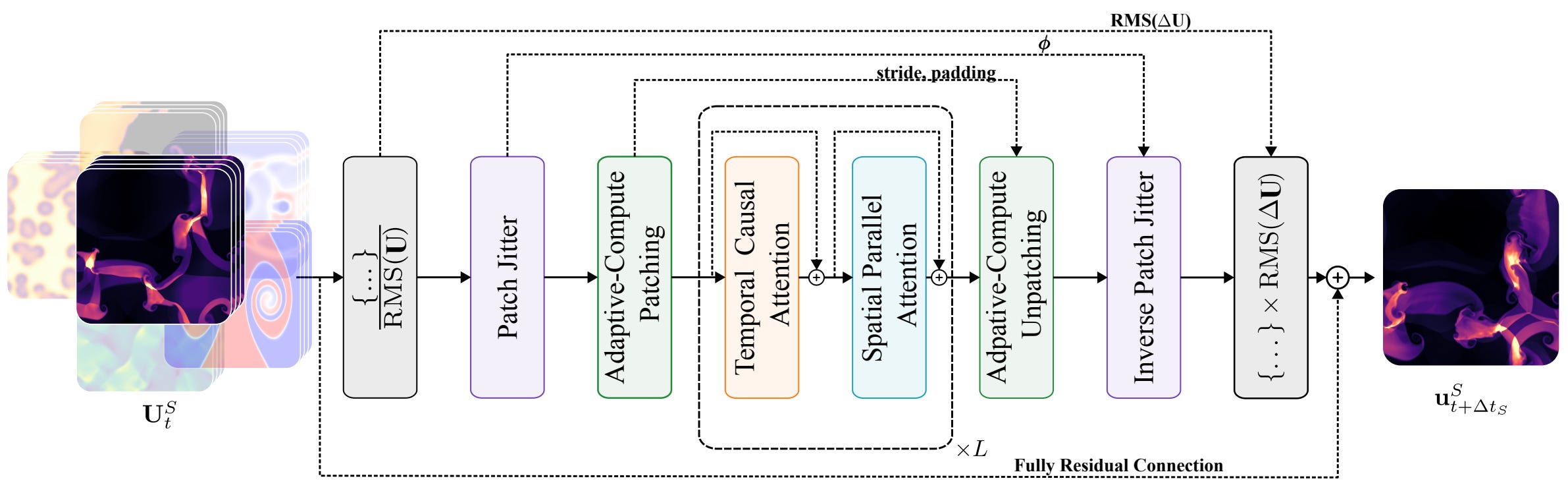
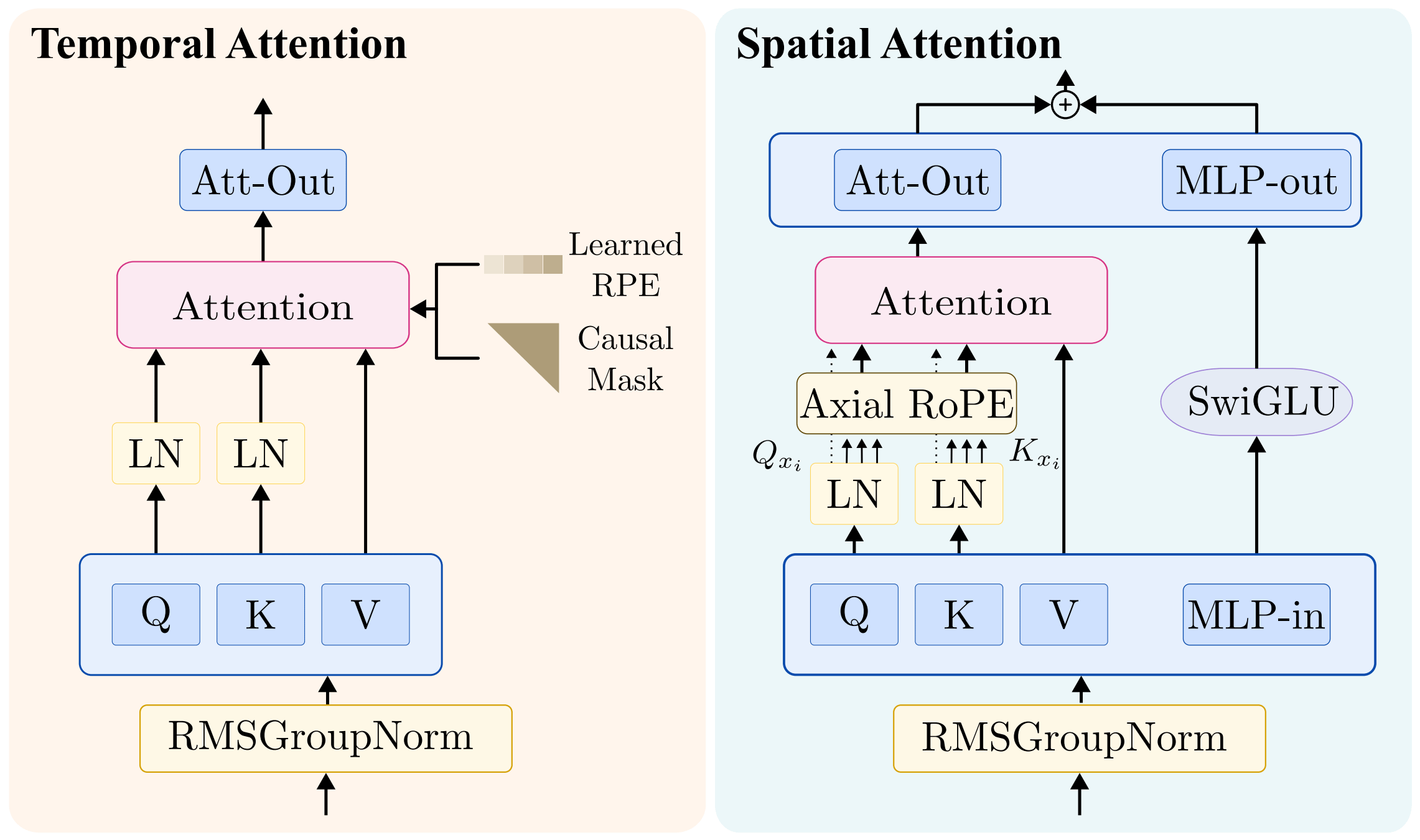
Walrus employs a space-time factorized transformer [2], that is a model alternating 1D attention operations between the time axis and the space axis. The axial attention in time is causal and uses a T5-style relative positional encoding that simply means that the model learns a bias B that is added to the attention matrix.
where M is the causal mask and Q, K , V linear pointwise transformation of the input.
While the attention applied on the space axis is not causal and adopts an Axial RoPE positional encoding.
Note that Q, K and V are not the same across the three attention modules. You can think about this factorized attention as a windowed attention, where the windows are ne-dimensional slices along the temporal, horizontal, and vertical axes, respectively.
Here a visualization of the attentions employed in Walrus:
Compute-Adaptive Compression
They adopt Convolutional Stride Modulation [3] in both encoder and decoder modules to natively handle data at varying resolutions by adapting the level of downsampling/upsampling in each encoder/decoder block.
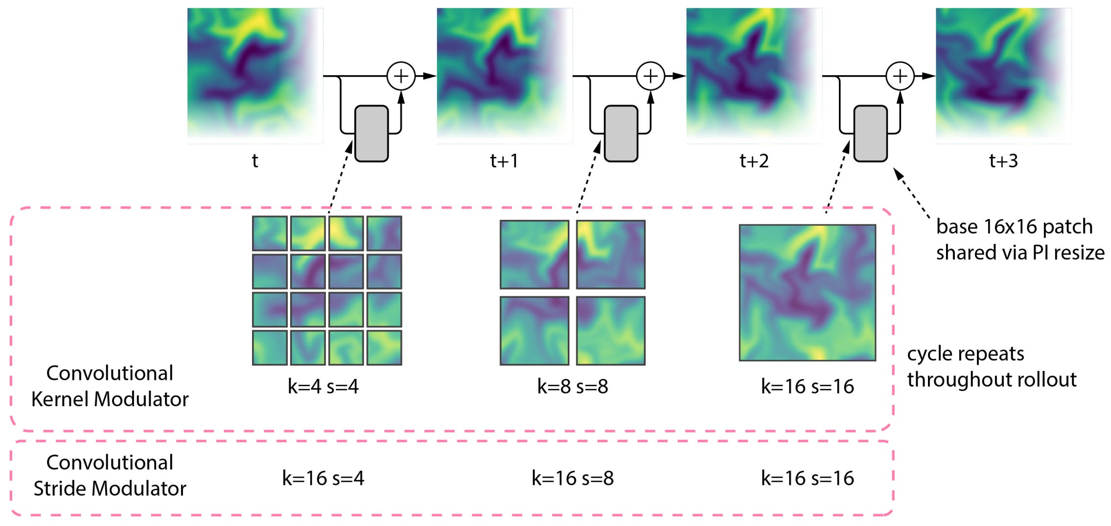
During pretraining, to maximize device utilization, they choosed a fixed number of tokens per axis and adjusted the downsampling factor accordingly such that data of the same dimensionality produces roughly the same number of tokens per frame across datasets.
Patch Jittering
Several studies have identidified one of the major contributors to the autoregressive instability in aliasing: The phonemenon of high freqency content folding into low-frequency bins.
In ViT-style architectures employing symmetric patchification or strided and transposed convolutions for tokenization/reconstruction can be particuarly noticeable s grid-like artifacts (we already observed that in the blog post on MANO, check it for some visualization of this phenomenon!)
Typically, we identify the non-linear activations as the major reason of aliasing. In Walrus, they shows that resampling operations of ViT-style models alone produce distinct spectral structure which leads to this grid-imprinting.
In short, considering a convolution g (used for downsampling), followed by a transpose convolution h (used for upsampling) by looking at his Fourier transform we observe that
where u is the input, v the output and P the ratio between the high resolution (before the conv) and the low resolution (after the conv).
We observe that the each output’s frequency becomes a weighted sum of the frequencies whose index is congruent modulo M. The weights are given by the kernel of the convolution and of the transposed convolution. This is exactly what creates the artifacts that you can see in the following image:
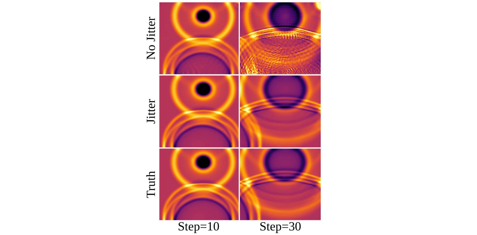
The authors realized that it’s possible to reformulate this process probabilistically by randomly translating the input data and inverting the translation in the output data. The expectation of this process leads to the un-aliased solution . In realistic settings, the expectation converges slowly but incorporating sampling without any averaging already provides significant benefits, at minimal cost (as you can check from the previous figure).
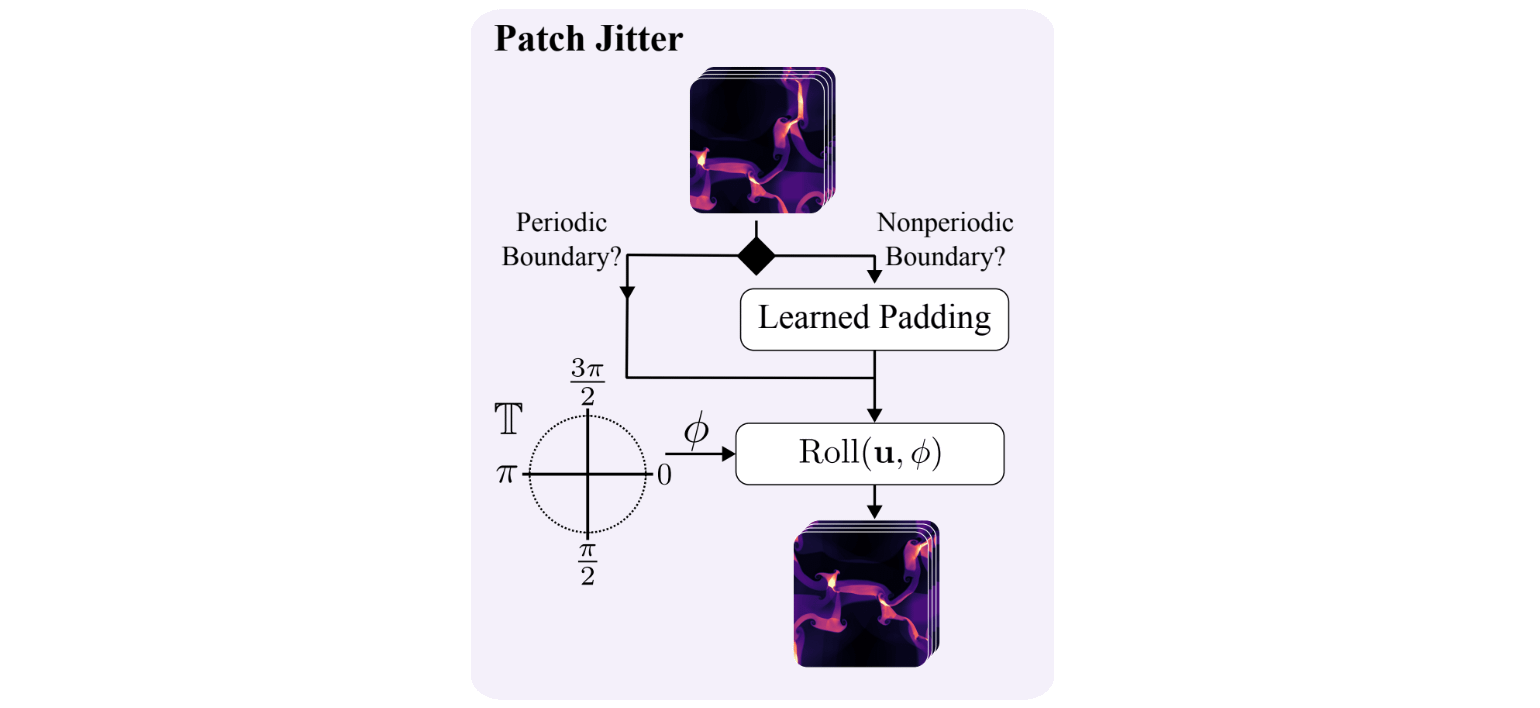
More in details, the Patch Jitter module first checks whether the input field satisfies periodic boundary conditions. For periodic data, the field can be shifted directly with a circular roll. For nonperiodic data, a learned padding operation is first applied so that the shift does not introduce artificial boundary discontinuities. A random angle is then sampled and used to determine the spatial displacement in the roll operation. The resulting randomly shifted field is finally passed to the patchification stage, so that patch boundaries change across training iterations.
Multi-Dimensional Inputs
A founduation model for physics is expected to handle data at different dimensionalities.
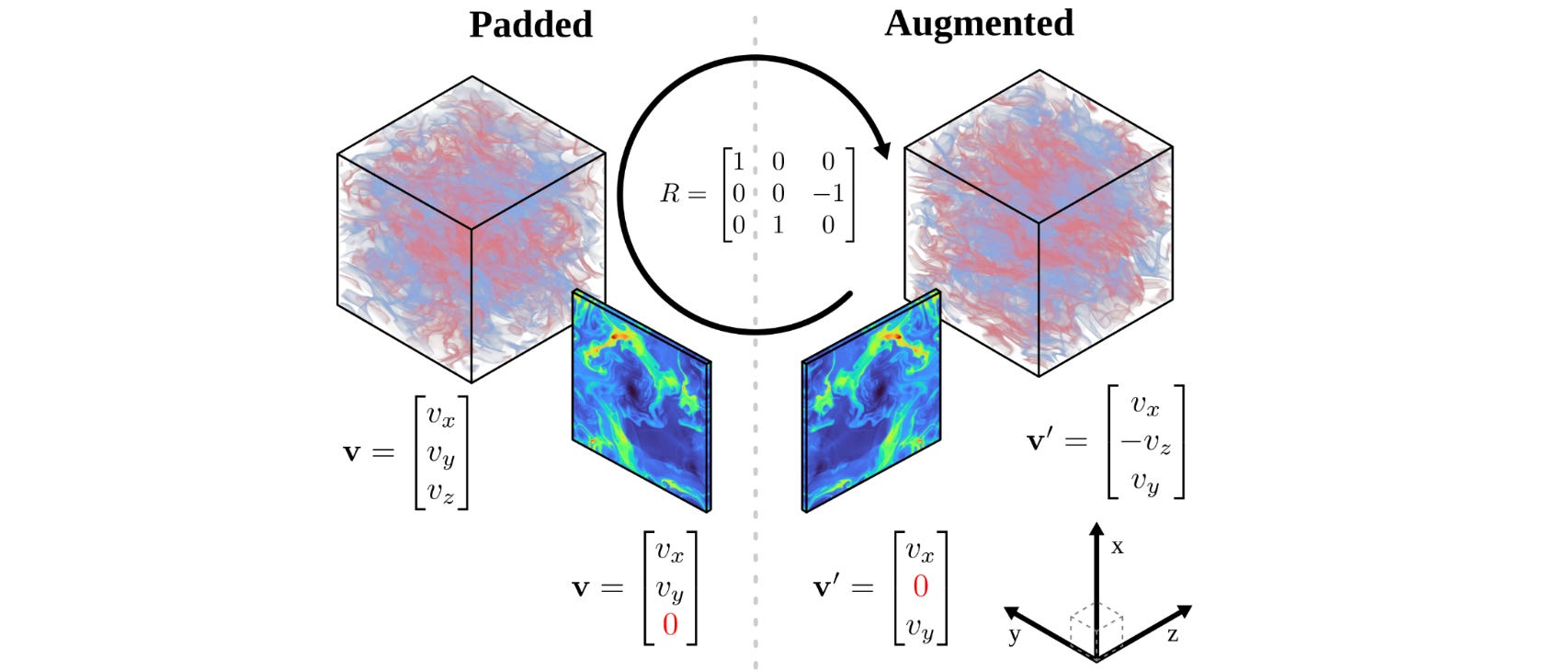
They are able to jointly handle 2D and 3D data in a single pipeline by treating 2D data as a thin plane randomly embedded in 3D space. The data is first projected into 3D by appending a singleton dimension and zero-padding the tensor-valued fields and then randomly rotated in 3D.
However, the 1D and 2D inputs use separate encoders and decoders, while inputs of the same dimensionality share these components. The architecture therefore contains two encoders and two decoders in total.
Conclusions
Walrus improves on previous models in several different ways. I did not go into the quantitative results here because I wanted to focus on the ideas and keep this blog post relatively short. Still, the results are really strong, and you can find all the details in the original paper.
There are also a few other interesting parts of the work that I did not cover, so I definitely recommend taking a look at the paper [1]. I think we will see many of the ideas discussed here appearing again in future scientific foundation models, and I am excited to see what the next iteration will look like.
One limitation I am particularly curious about is that Walrus does not currently handle irregular meshes. I am already waiting for a point-cloud version!