
13. Multi-branch transformers with AB-UPT
How to model different physical quantities with different parts of the model while keeping information sharing between them.

Introduction
This blog post is about multi-branch transformer architectures, we will discuss in details how in Anchor-Branched (AB) -Universal Physics Transformer (UPT), they designed a model that have different branches for different physical quantities, how they made attention more efficient and how they enforced physics consistency.
We discussed in previous blog posts UPT and NeuralDEM. UPT is a strong Transformer-based model for physics: instead of applying attention directly on all mesh or point-cloud nodes, it first compresses the input into a latent space through message passing to randomly sampled nodes, called supernodes, and then applies Transformer layers in this compressed representation.
NeuralDEM builds on this idea and introduces a multi-branch Transformer structure, specialized for predicting the dynamics of a large number of particles interacting with a fluid. AB-UPT can be seen as a further development of these ideas: it keeps the latent Transformer philosophy of UPT, takes the multi-branch direction more seriously, and adapts it to large-scale aerodynamic problems with multiple physical output quantities. Let’s start!
The problem
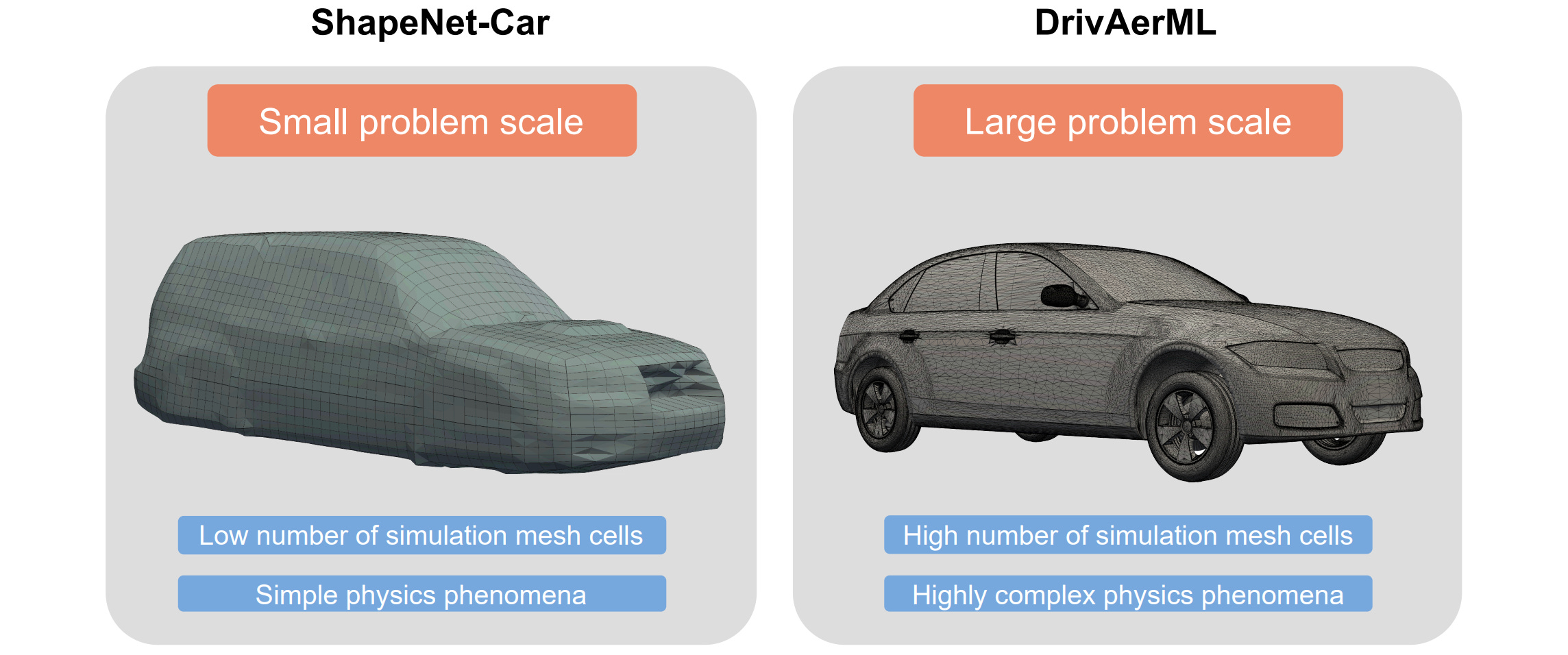
The problem they consider is CFD simulation of automotive aerodinamics: more concretely, you are given the shape of a car (called car geometry) and you want to predict quantities on its surface (such as the pressure) and on the 3D volume around the car (e.g. velocity and pressure fields, turbulence related quantities) as well as global quantities such as drag and lift. Here a sample of car’s geometry from two common datasets:
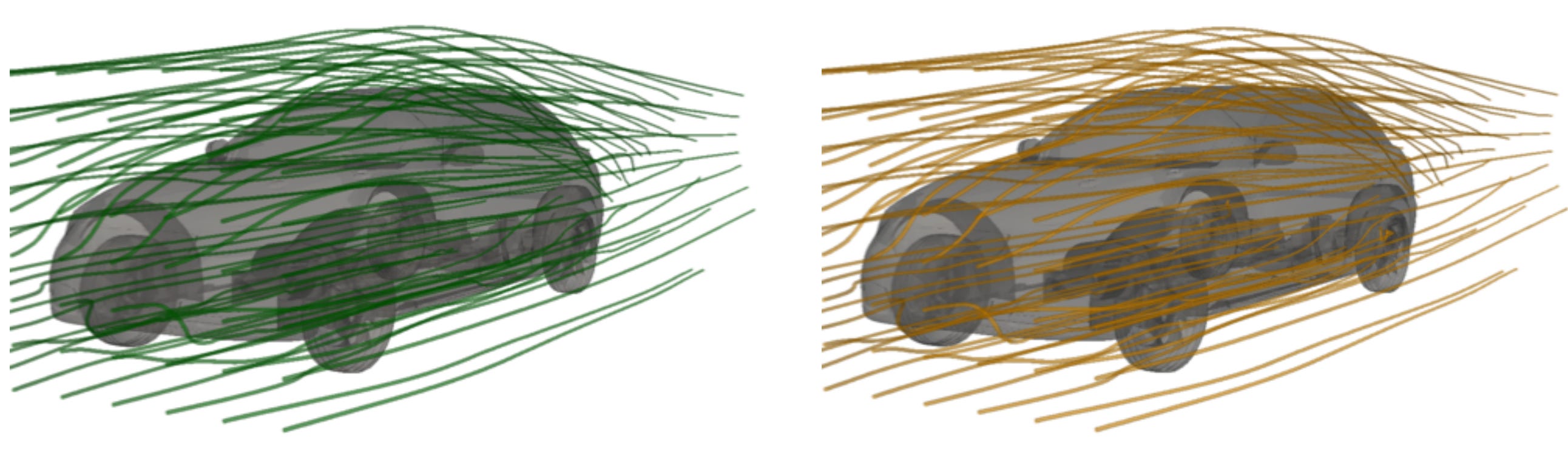
And here a sample of velocity streamlines (a streamline is a curve always tangent to the velocity field):
These problems typically contains very big meshes (e.g. 140 Million points per sample in DrivAerML) and this resolution is necessary for engineering applications. Therefore, scaling is a main point of interest in AB-UPT.
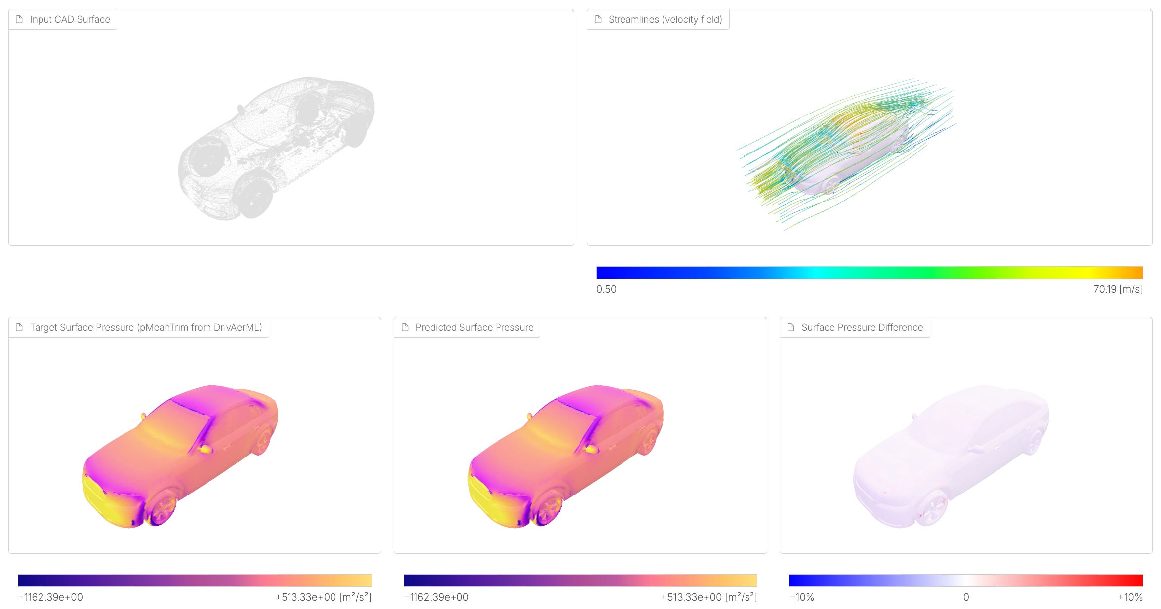
Here an example of high resolution prediction of AB-UPT:
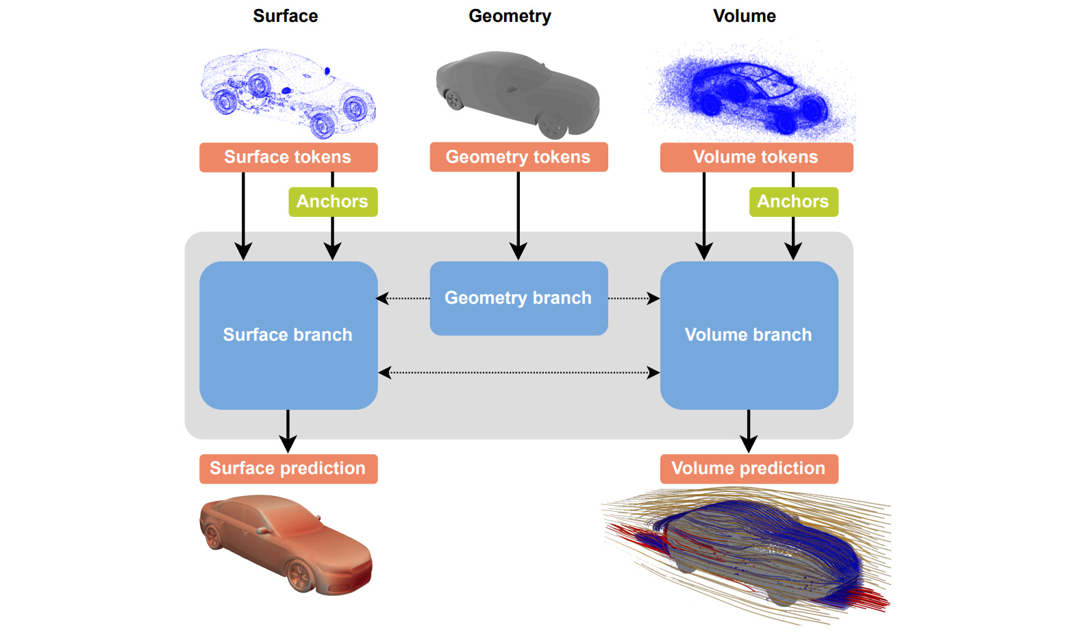
Multi-branch design
The model is organized into 3 branches:
Geometry-encoding
Surface-prediction
Volume-prediction
In short, each branch contains its own tokens, and tokens within the same branch interact through self-attention. This allows the model to process each type of information in a specialized way: the geometry branch builds a representation of the input shape, the surface branch predicts quantities defined on the object surface, and the volume branch predicts quantities in the surrounding flow field. The important point is that the model does not treat all physical quantities as one homogeneous output. Instead, it separates them into different computational paths, while still allowing information to be shared between branches through cross-attention mechanisms. Let’s dive into the details!
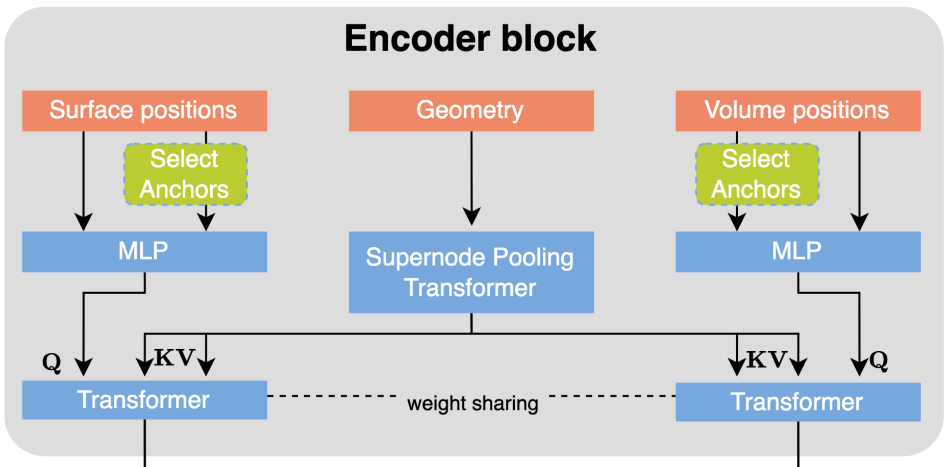
Multi-branch encoder
The encoder start with a supernode pooling Block that maps the input geometry M into a reduced set of supernode representations via message passing with a fixed radius. Interestingly, this is the same supernode pooling used in UPT with the difference that here is applied just to the geometry and not to the physical fields.
The resulting supernode representations are passed through a self-attention block, allowing the supernodes to aggregate global information from the other supernodes, resulting in the output of the geometry branch.
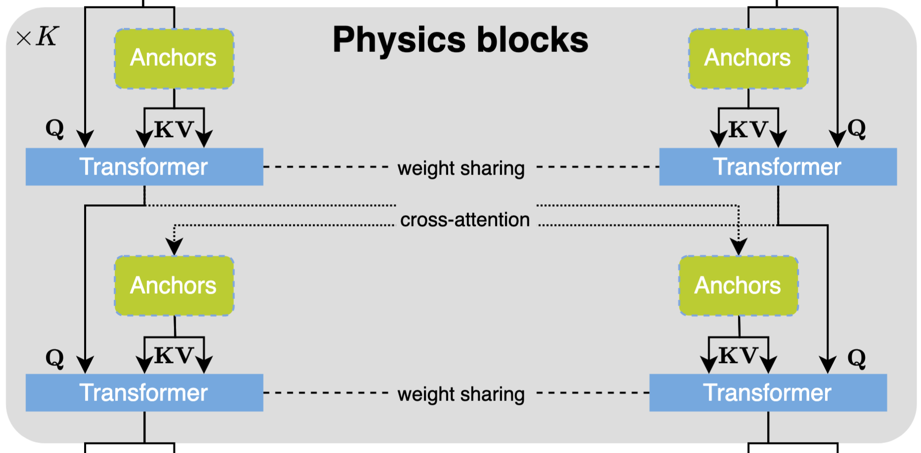
Multi-branch blocks
To bridge the geometry and the surface and volume branches, AB-UPT uses a cross attention (Queries are generated from the surface/volume branch while Keys and Values are obtained from the output of the geometry branch). The 2 cross-attention of surface and volume branches share parameters.
Each AB-UPT block consists of a self-attention and cross-attention block, which, again, share parameters between the surface and volume branches.
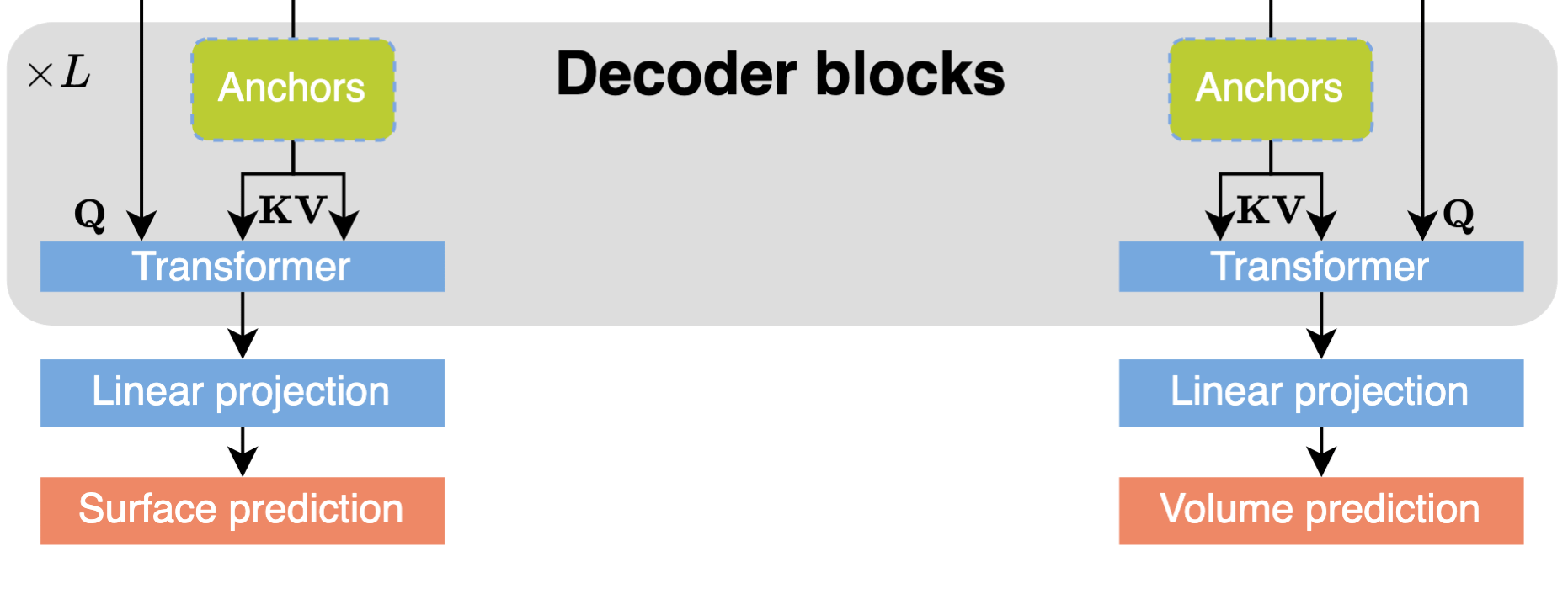
Multi-branch decoder
The final decoder block consists of several self-attention blocks that do not share parameters and hence operate independently. The query, key, and value representations all originate from the previous layer, and, therefore, there is no interaction anymore between the two branches. This design allows for branch-specific modeling, meaning each branch can refine the output predictions independently, without interaction with the other branches.
Finally, a single linear projection is applied as a decoder to generate the final output predictions for each branch.
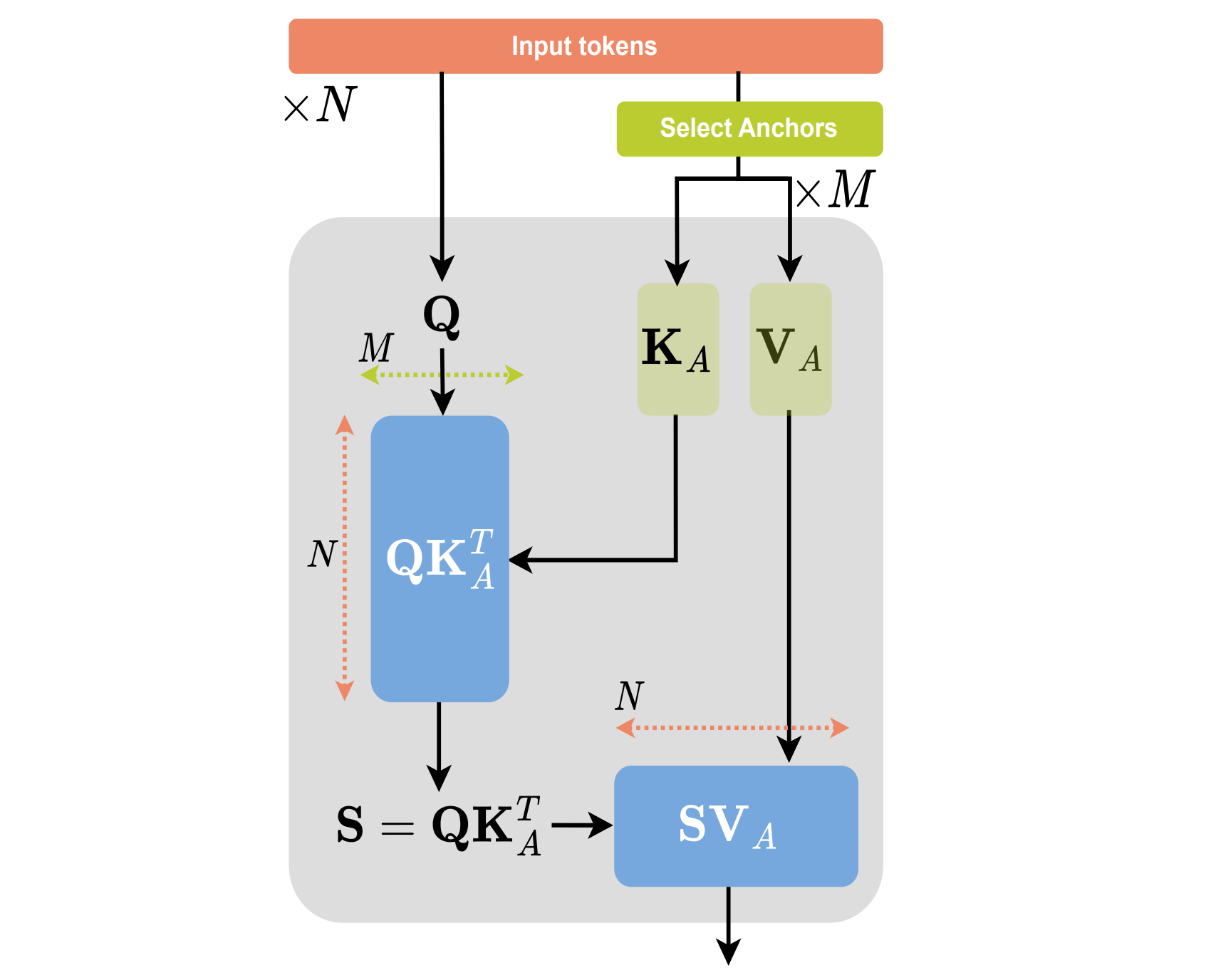
Anchor Attention
In the previous chapter, to simplify the explanation, we committed a small lie (that you might have already spotted from the previous figures). In AB-UPT, the authors do not use standard cross-attention directly between all simulation points, because this would have quadratic complexity in the number of points and would quickly become too expensive at large scale. Instead, they introduce what they call Anchor attentoin, from which the “A” of AB-UPT.
Anchor attention, randomly selects a subset of the points called Anchors from which the Key and Value matrices are computed for the attention while the Query matrices are obtained from the full sample (actually part of the sample, depending on the branch!). Doing so, the anchor attention has complexity O(MN) where M is the number of anchor tokens and N the number of query tokens.
The way I see it is as an extension of the supernodes idea. Instead of simulating completely in a coarse latent space, AB-UPT simulates in the full space of supernode-like tokens, while keeping the heavy operations on a coarser latent space, given by the anchor points. As a consequence, at same computational budget, AB-UPT can afford a larger latent space of supernodes than UPT.
By treating the anchors as conditioning set for the queries, anchor attention turns the architecture into a conditional field model: the field values at any query location are predicted from the query location itself and the context provided by the anchors, but independently from any other query location.
Enforcing physics consistency
Another interesting ingredient of AB-UPT is the way it enforces physics consistency.
Instead of asking the model to directly predict vorticity as a completely free field, the authors exploit a simple but important physical identity: vorticity can be written as the curl of a velocity field:
and therefore its divergence must be zero. In other words,
by construction. This is quite elegant because the model does not need to learn this constraint from data, neither it’s only softly encouraged through an additional loss term. The architecture is designed so that the predicted vorticity is divergence-free automatically.
Practically, AB-UPT outputs a continuous neural field, evaluates it around each query point, and computes the curl using finite differences. This makes the model slightly more expensive, but it gives a hard physical guarantee.
A surprising phenomenon
Something that surprised quite a lot the first time I read this paper was Table 4:
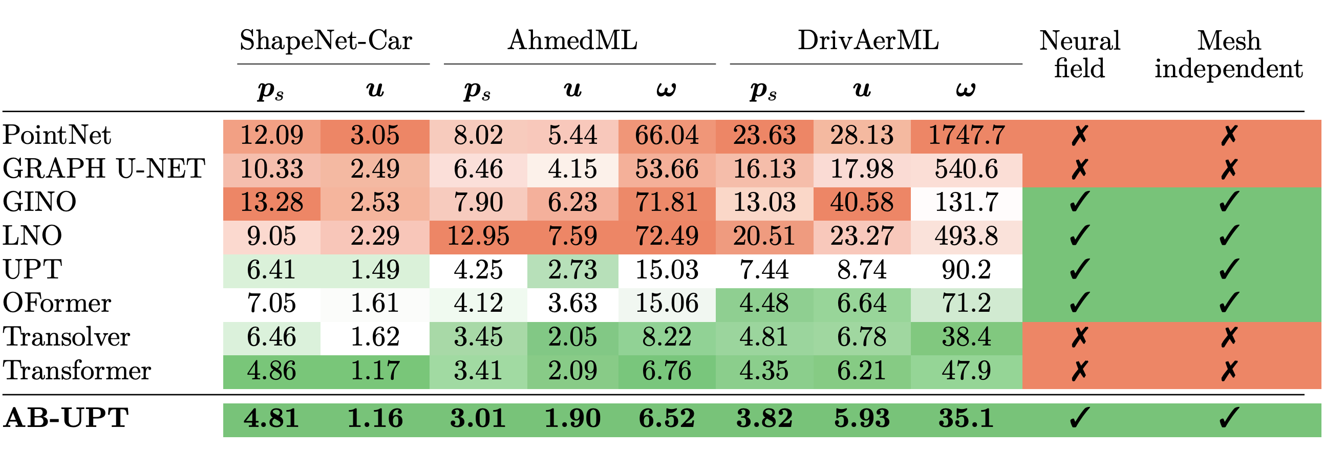
Did you notice anything strange? AB-UPT is the best overall, and that is expected. But very close, in second position, there is “Transformer”.
What is this?
Well, it’s a plain Transformer, pretty much the same of the one presented by Vaswani et al. back in 2017. Interestingly, when trained with modern recipes and properly optimized, it is still one of the strongest models. To be fair, it is quite slow, around 100x slower than AB-UPT and slower than other Transformer-based baselines such as Transolver, but still, its performance is surprisingly competitive.
Conclusions
AB-UPT has introduced many interesting features, I’m genuinely curious to see what the community will build on it and what will be the next Emmi AI’s iteration. Of course, I’ll keep you updated!