
11. Universal Physics Transformer (UPT)
A framework for efficiently scaling neural operators.

Introduction
In the last blog post we discussed about Aurora, the first foundation model for the atmosphere. Among the authors figures Johannes Brandstetter, that after his experience at Microsoft, came back to Austria with a faculty position and co-founded the start-up, Emmi AI, that is leading Transformer based approaches for numerical simulations in engineering. Their first model was the Universal Physics Transformer (UPT). As we will see, this model builds upon the Aurora project but with many innovations that enabled the strong performances at scale that we will discuss soon.
They tried to answer a simple, yet necessary, question:
what is an efficient way to scale neural operators to larger and more complex simulations, by taking into account different types of simulation datasets?
The need for a unified architecture
For a model for physics, to be called a “foundation model”, it needs to be able to address the two opposite type of simulations: Eulerian and Lagrangian simulations. This is not an exhaustive classifications of all numerical simulations but these two classes includes the vast majority of them.
Eulerian simulations
Eulerian schemes monitor the physical field of interest (such as velocities) at specific fixed grid points. These points, represented by a spatially limited number of nodes, control volumes, or cells, serve to discretize the continuous space. This process leads to grid-based or mesh-based representations. This is, in my opinion, the most classical type of simulations.
Lagrangian simulations
in Lagrangian schemes, the discretization is carried out using finitely many material points, often referred to as particles, which move with the local deformation of the continuum. In lagrangian simulations, instead of observing the system at fixed spatial locations, you follow individual particles or material points.
The architecture
UPT brought two main innovations:
An encoder-decoder strategy that enable to query the output at any point
Latent rollout for efficient long-range time predictions.
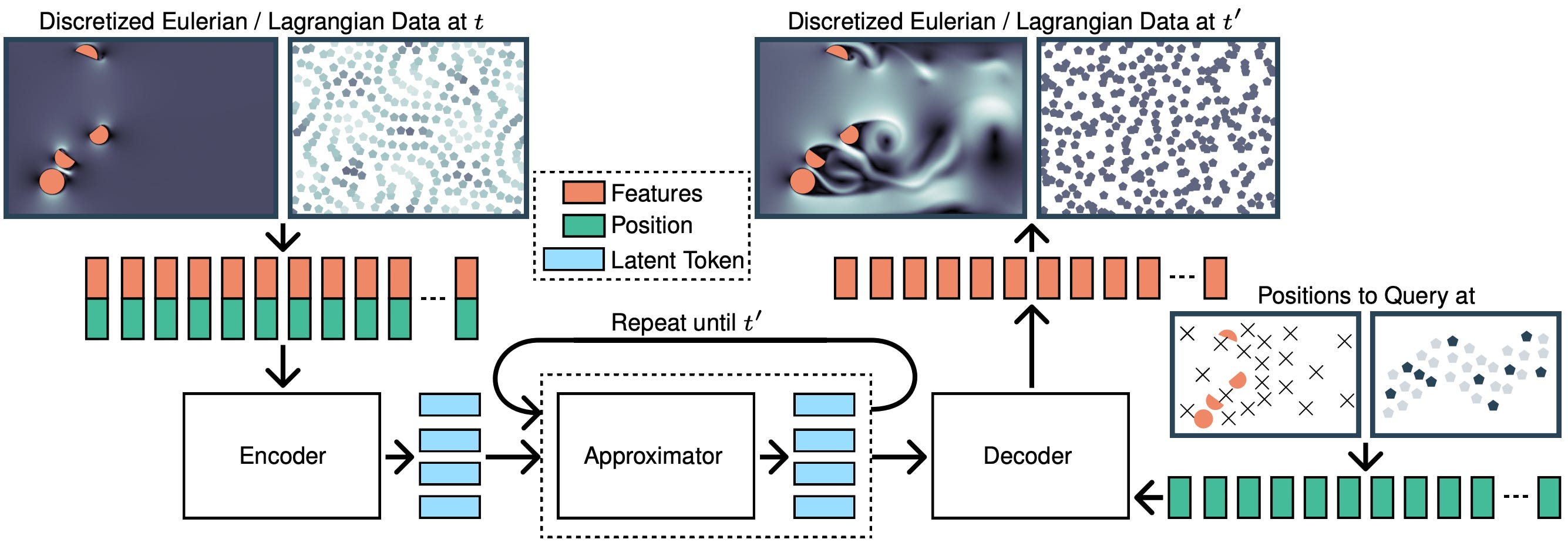
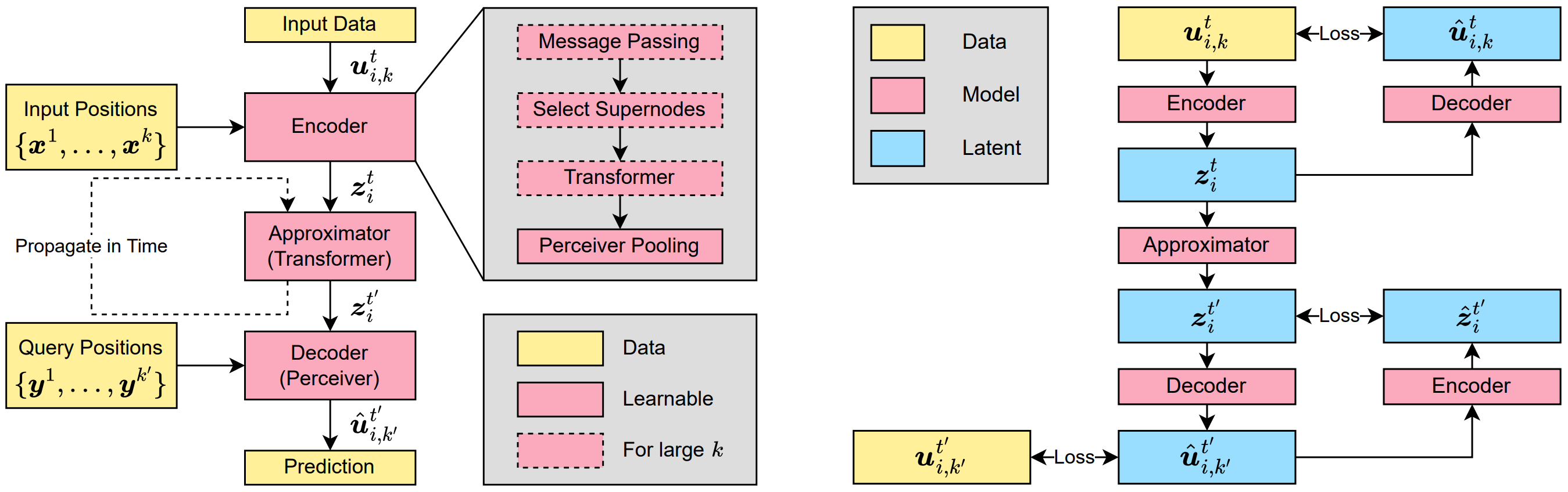
As usual, the model has an encoder-approximator-decoder structure:
Encoder
The goal of the encoder is to compress the input signal, represented as a point cloud, selectively focusing on the important parts of the input.
The encoder firstly selects n points among the point cloud input randomly (that can be seen as an importance sampling of the underlying simulations since it allocates more supernodes to highly resolved areas in the mesh or densely populated particle regions, this analogy holds provided that the mesh used for the simulation is already good enough) and information is exchanged between locally between points and supernodes via a message passing layer. The super nodes are then feeded to a perceiver model (as we already saw in Aurora!) that is an attention module where keys and values are obtained from the layer’s inputs (here the super nodes) while the queries are learned parameters.
if an application requires a variable sized latent space, one could also remove the perceiver pooling layer. With this change the number of super nodes is equal to the number of latent tokens and complex problems could be tackled by a larger super node count.
Approximator
The approximator propagates the compressed representation forward in time.
They adopted a standard transformer as approximator. Crucially, this is computationally fine since the latent representations are much smaller than the input so the quadratic complexity (in the mesh size) of attention is not a big issue.
Decoder
The task of the decoder is to query the latent representation at any set of arbitrary locations.
They enabled the model to query the output function anywhere by using a perceiver module where, this time, the queries are an embedding of the output positions, instead of learnable parameters as in the encoder. More concretely, the output positions are passed through an MLP to produce the query matrix.
Model conditioning
To condition the model to the current time-step and to boundary conditions, they added feature modulation to all transformer and perceiver blocks, they employed a FiLM modulation (the same used in diffusion transformers (DiTs)) which consists of a dimension-wise scale, shift and gate operation that are applied to the attention and MLP module of the transformer. Scale, shift and gate are dependent on an embedding of the timestep and boundary conditions.
Latent rollout
During the autoregressive rollout, the field must be decoded and re-encoded at every time step for the next prediction. This is computationally costly. Therefore, in UPT they introduce latent rollout, which consists of propagating the field forward in time directly in the latent space, without decoding and re-encoding at each step. For this to be possible, the encoder and decoder must form an autoencoder (i.e., the decoder must be the inverse of the encoder). This is enforced by adding two reconstruction losses: one for the left inverse, Decoder(Encoder(z)) = z, and one for the right inverse, Encoder(Decoder(z)) = z.
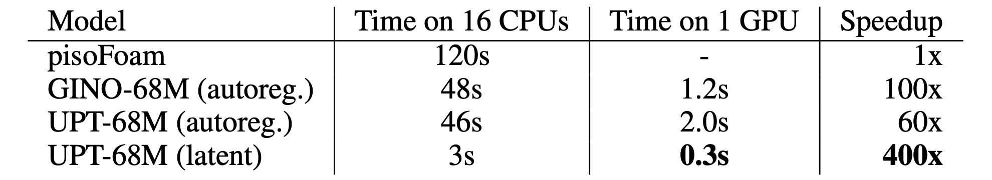
The latent rollout is more than 5x faster than an autoregressive rollout via the physics domain:
Conclusions
UPT was one of the very first transformer-based models able to scale to a level close to industrial fluid dynamics simulations. In the next episodes of this blog series, we will look at follow-up works proposed by the same team. These models are highly capable of handling engineering simulations at an industrial scale.
UPT was the first paper I read during my PhD. Suggested by my supervisors and some friends of him, it was a great starting point. We did not work on a follow-up ourselves, as the required scale is prohibitive with typical academic computational resources but I’ve learned a lot by reading it and I would recommend to anyone starting research in this area to give a close look at the original paper [1].